Babaev — Forecasting Intermarket Dependencies

▶ Live Investor Signal Demo

Run the thesis models in real time — directly in your browser. Adjust market conditions and watch the AR1 dependency forecast and stress classifier respond instantly. Try the historical scenario presets to see how the signal would have fired during real market events.

Forecasting model

AR1 · RMSE=0.0659 · R²=0.9424

Signal classifier

Logit · F1=0.243 · AUC=0.532

Historical scenario presets — click to load

Typical trading day — BTC showing moderate positive correlation with S&P 500, normal volatility, no strong directional momentum.

Adjust Market Conditions

BTC–S&P500 Rolling Correlation (30-day) 0.35

−1 fully inverse0 uncorrelated+1 co-moving

Today's BTC Daily Return 0.0%

−20% crash0% flat+20% rally

BTC 20-day Annualised Volatility 55%

20% calm55% typical150% extreme

BTC 5-day Momentum (rolling return) 0.0%

−40% downtrend0% flat+40% uptrend

How it works

STEP 1

AR1 forecasts tomorrow's BTC–S&P500 dependency using today's Fisher-z correlation

STEP 2

Logistic regression combines the forecast + crypto features to estimate stress probability

STAY IN MARKET

Low stress probability — dependency stable

0.368

Current dep. (Fisher-z)

0.364

Tomorrow's forecast

Stress Probability 12.4%

0% 30% alert 60% exit100%

Low stress probability. Maintain normal equity exposure. Monitor for BTC volatility increases.

Recommended action

Hold current equity positions. No risk reduction needed based on crypto signal.

Educational demo — not financial advice. Coefficients are approximate, derived from walk-forward OOS evaluation 2020–2026 on 3,053 daily observations.

Dataset & Asset Universe

Asset Universe — Detailed

BTC-USD

Bitcoin

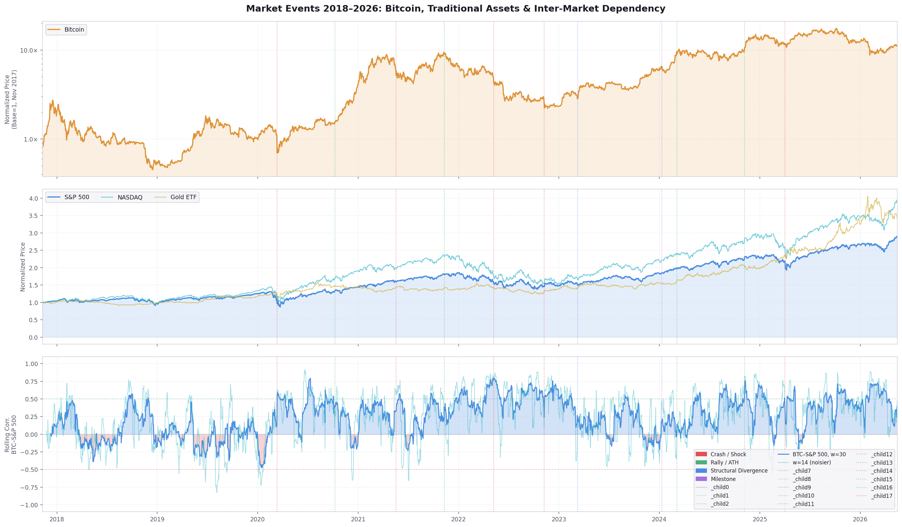
Base asset. World's largest cryptocurrency by market cap. Trades 24/7 including weekends. Serves as the primary source of crypto-derived features throughout the thesis.

Base crypto

ETH-USD

Ethereum

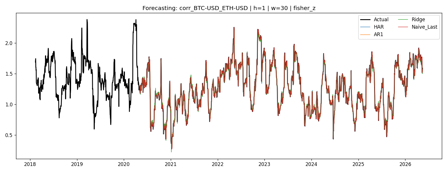
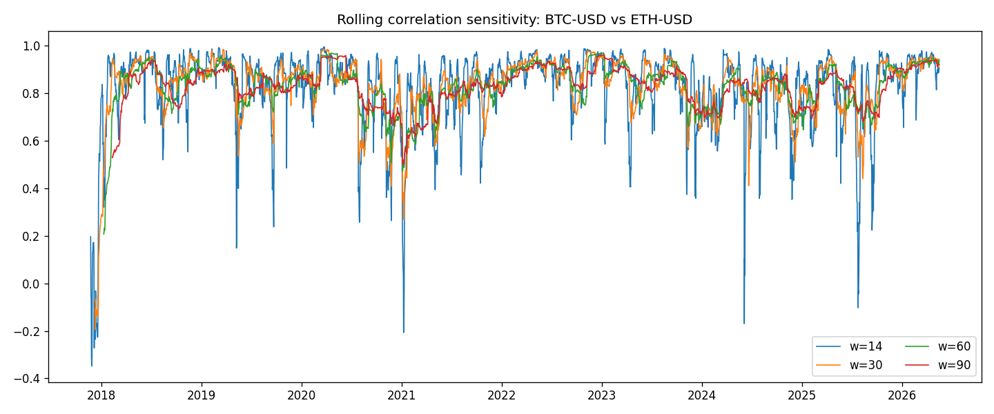
Crypto reference asset. Included to contrast cross-crypto dependency (BTC↔ETH) with crypto-to-conventional dependency. Start date of sample determined by ETH availability on Yahoo Finance.

Crypto ref.

^GSPC

S&P 500 Index

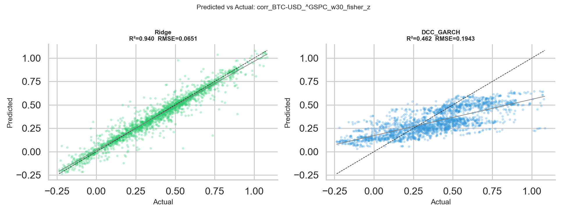
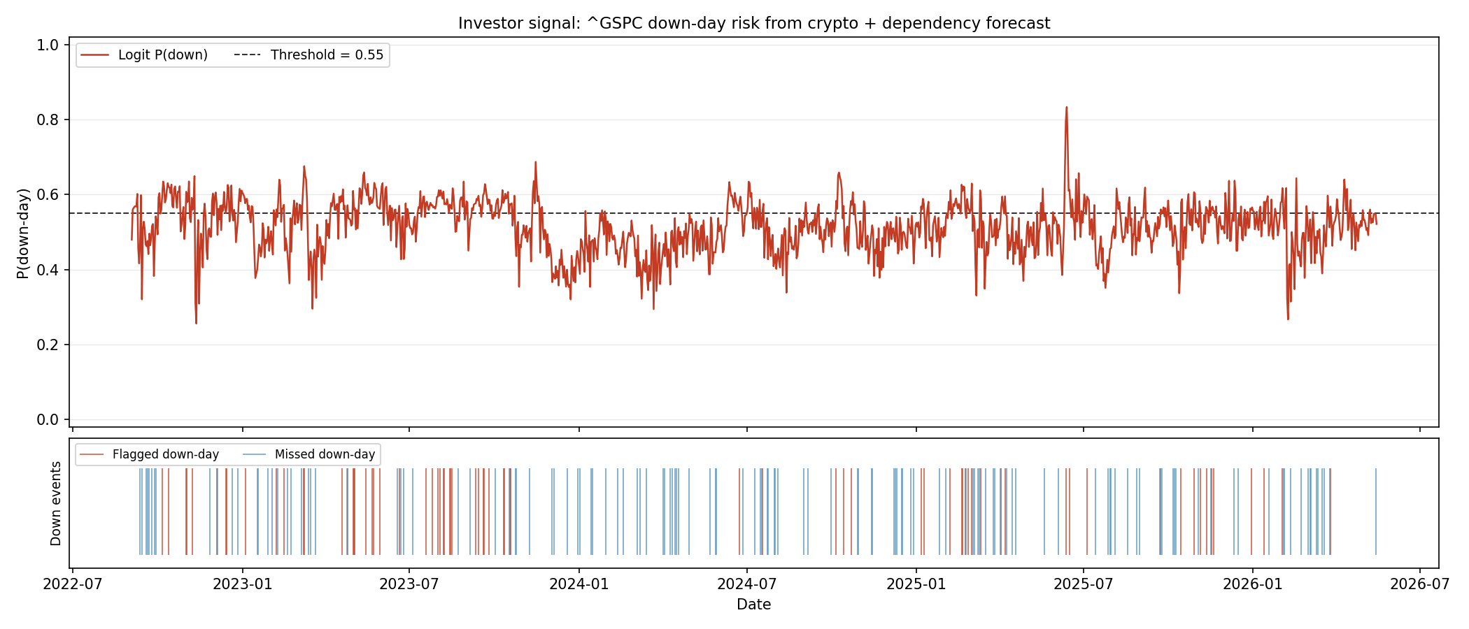
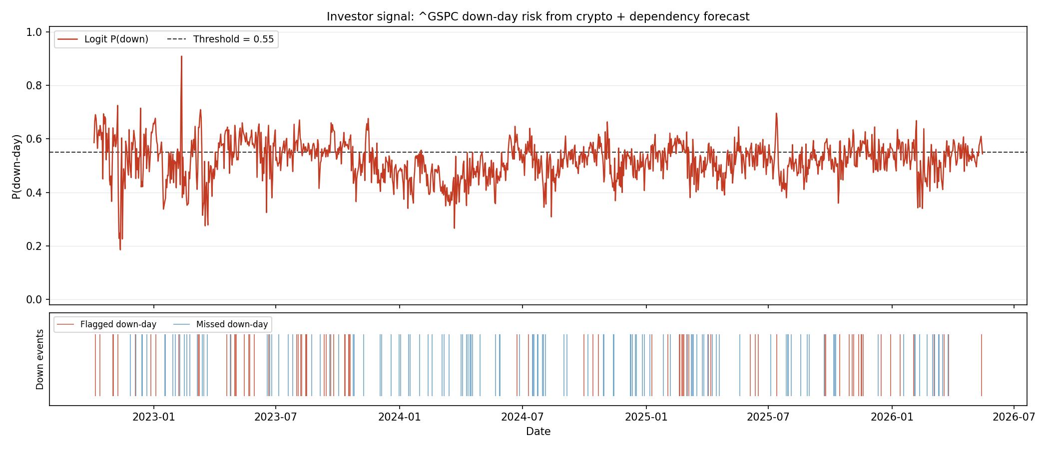
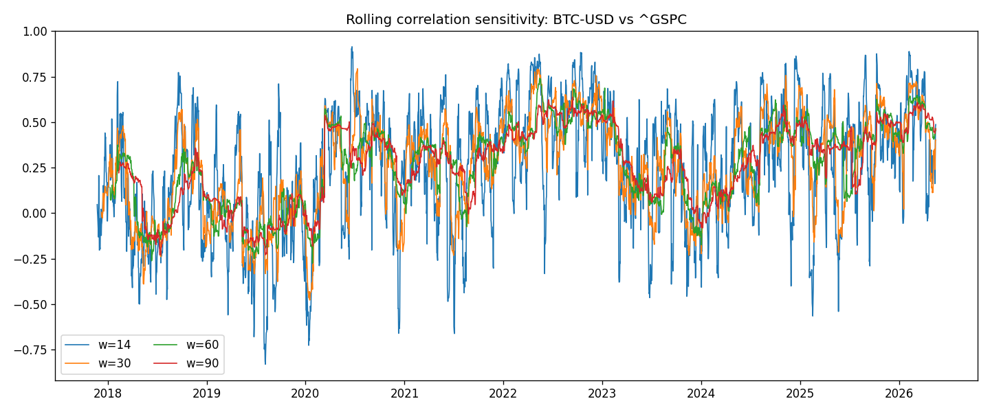
Broad U.S. equity benchmark. Represents large-cap risk appetite; most tightly linked to global funding conditions and sentiment — the same macro forces that drive Bitcoin.

Equity

^IXIC

NASDAQ Composite

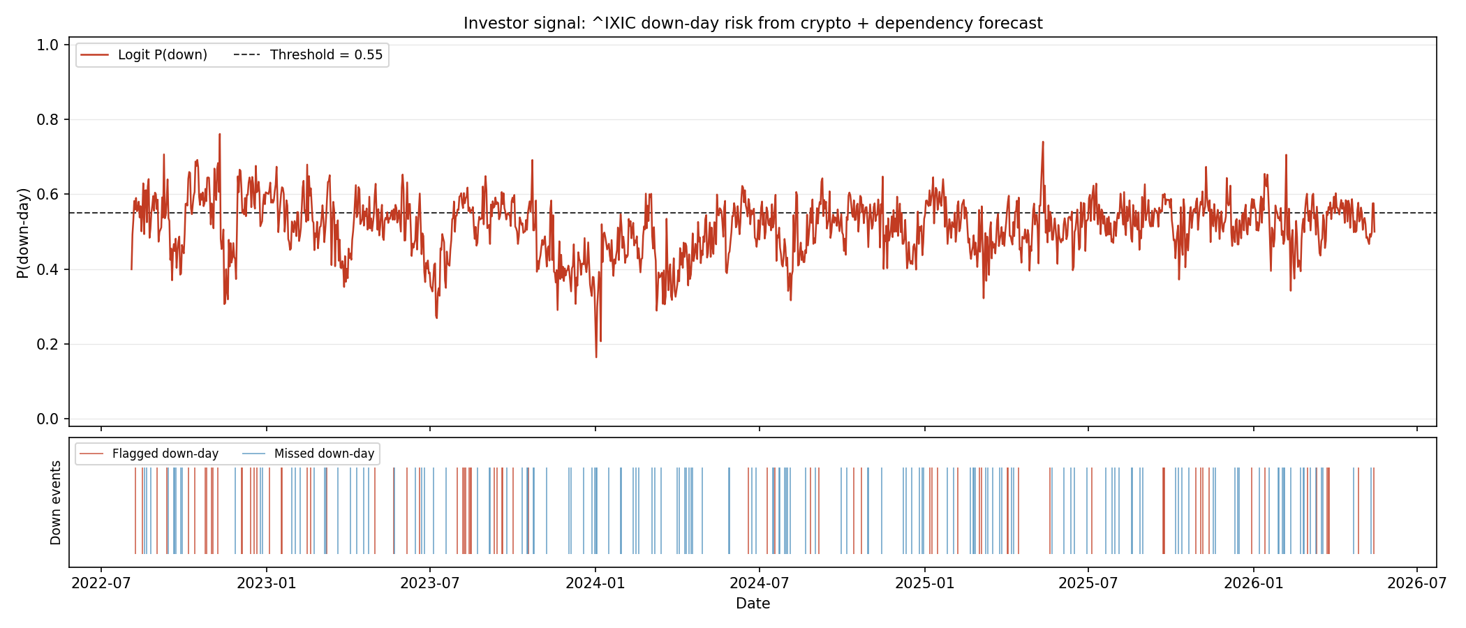
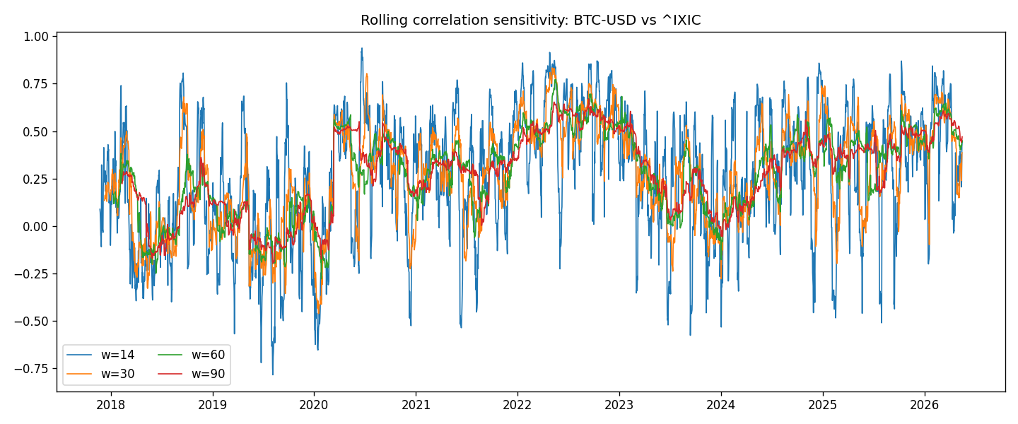
Tech-heavy equity index. Higher beta to growth and speculative sentiment than S&P 500, making it a natural comparator for crypto co-movement.

Equity

GLD

SPDR Gold Shares ETF

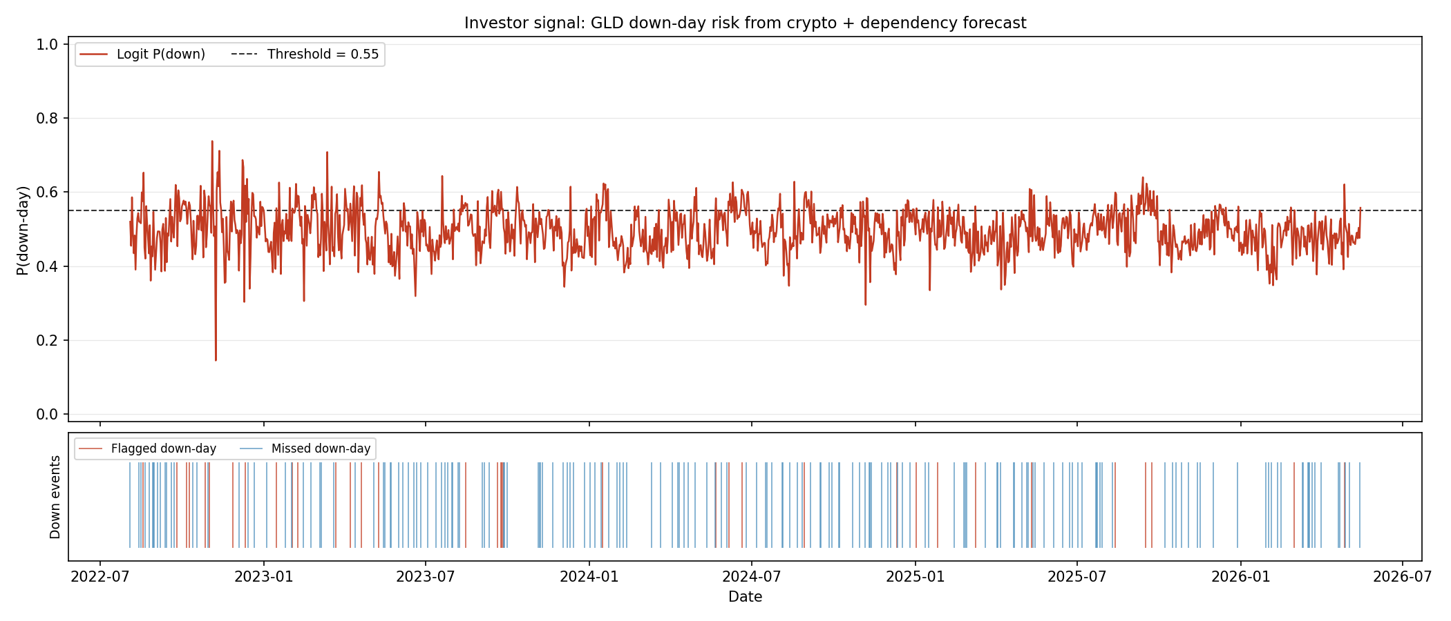
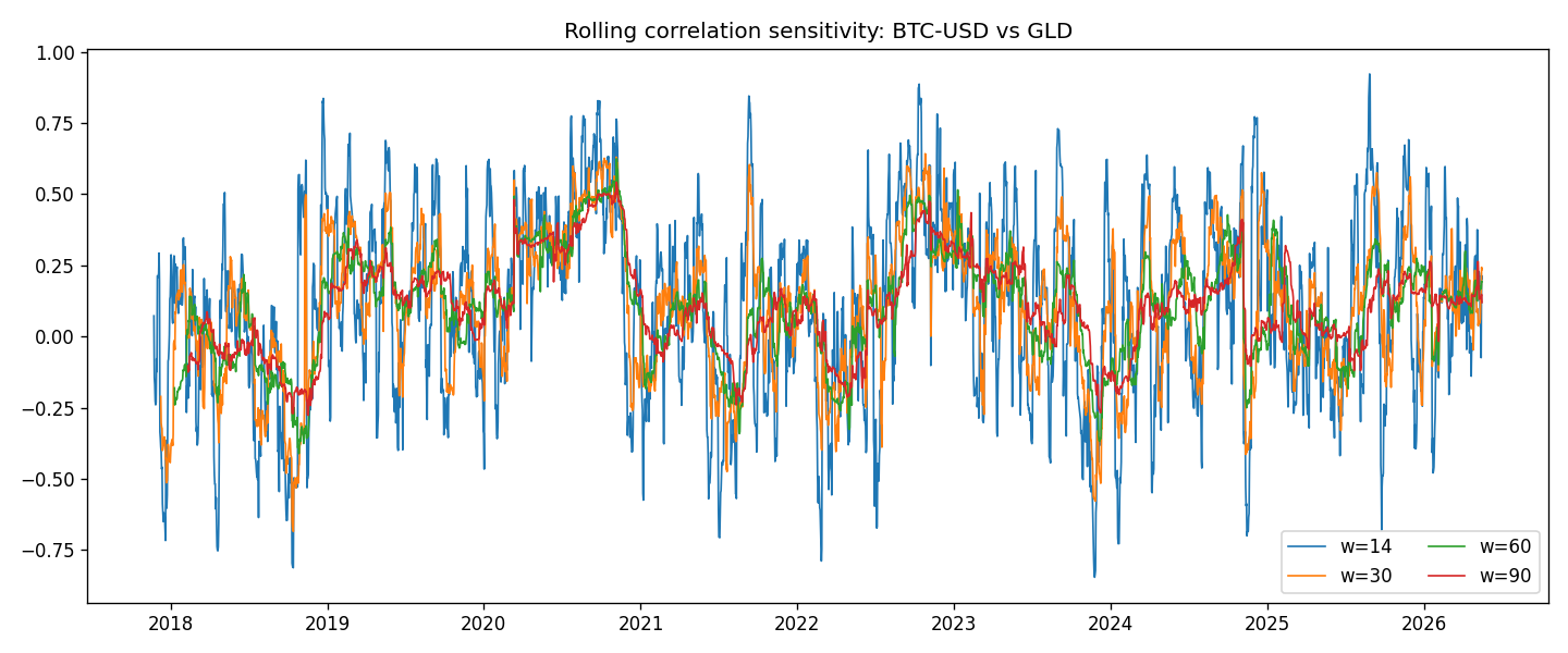
Largest gold ETF. Captures safe-haven demand, inflation expectations, and real interest rate dynamics — structural drivers distinct from crypto.

Precious metal

SLV

iShares Silver Trust ETF

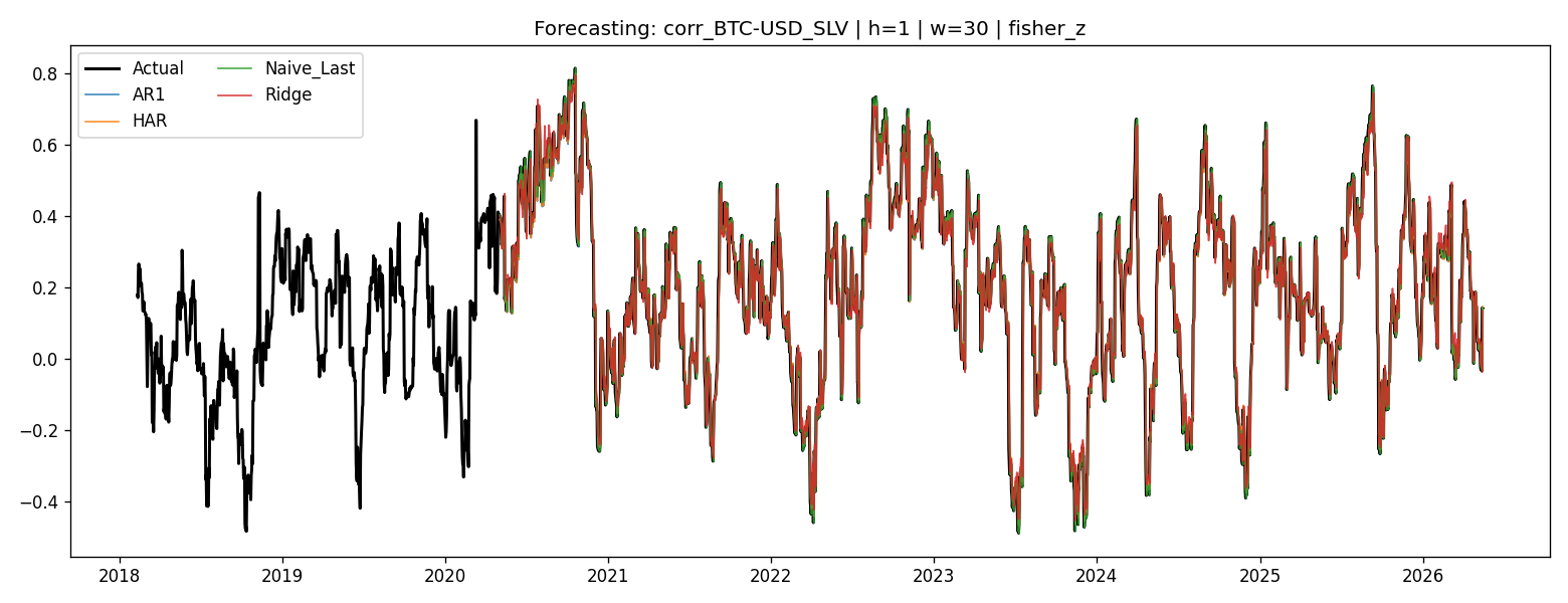
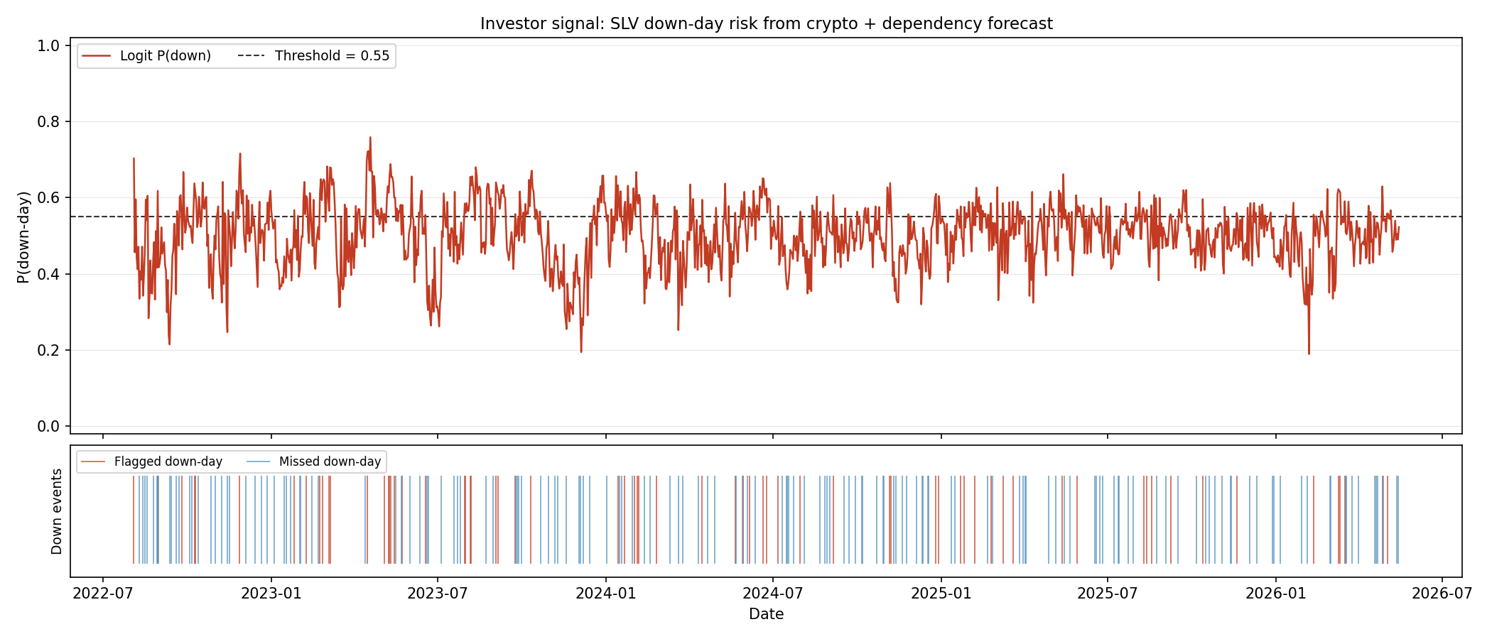
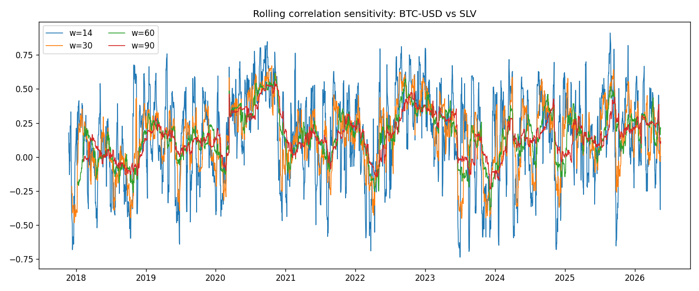
Silver has both safe-haven and industrial demand components. Higher volatility than gold; provides an additional precious-metal data point.

Precious metal

UUP

Invesco US Dollar Index ETF

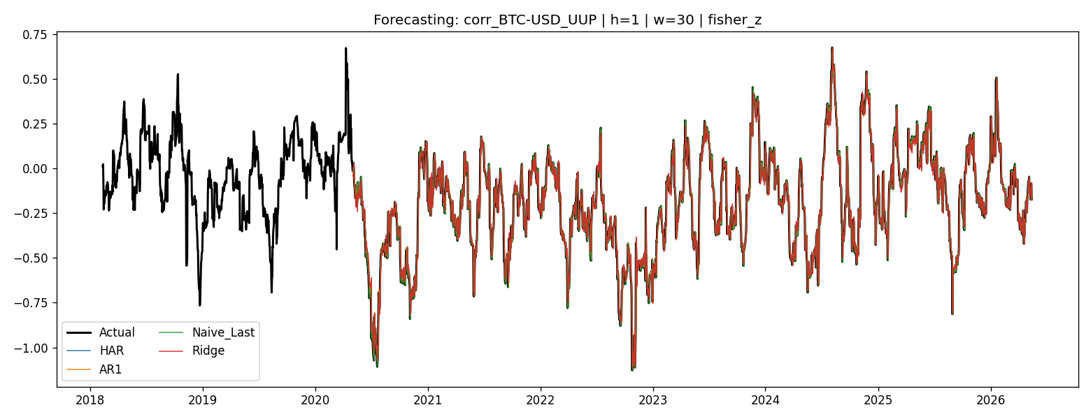
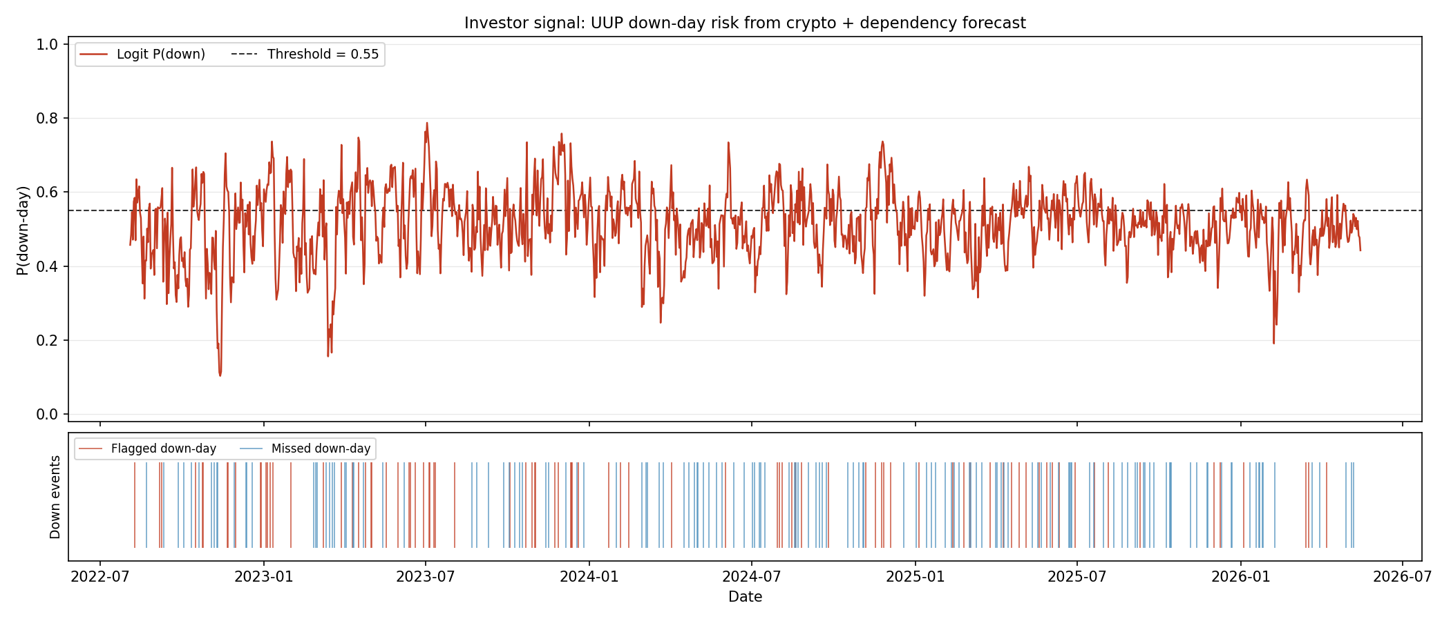
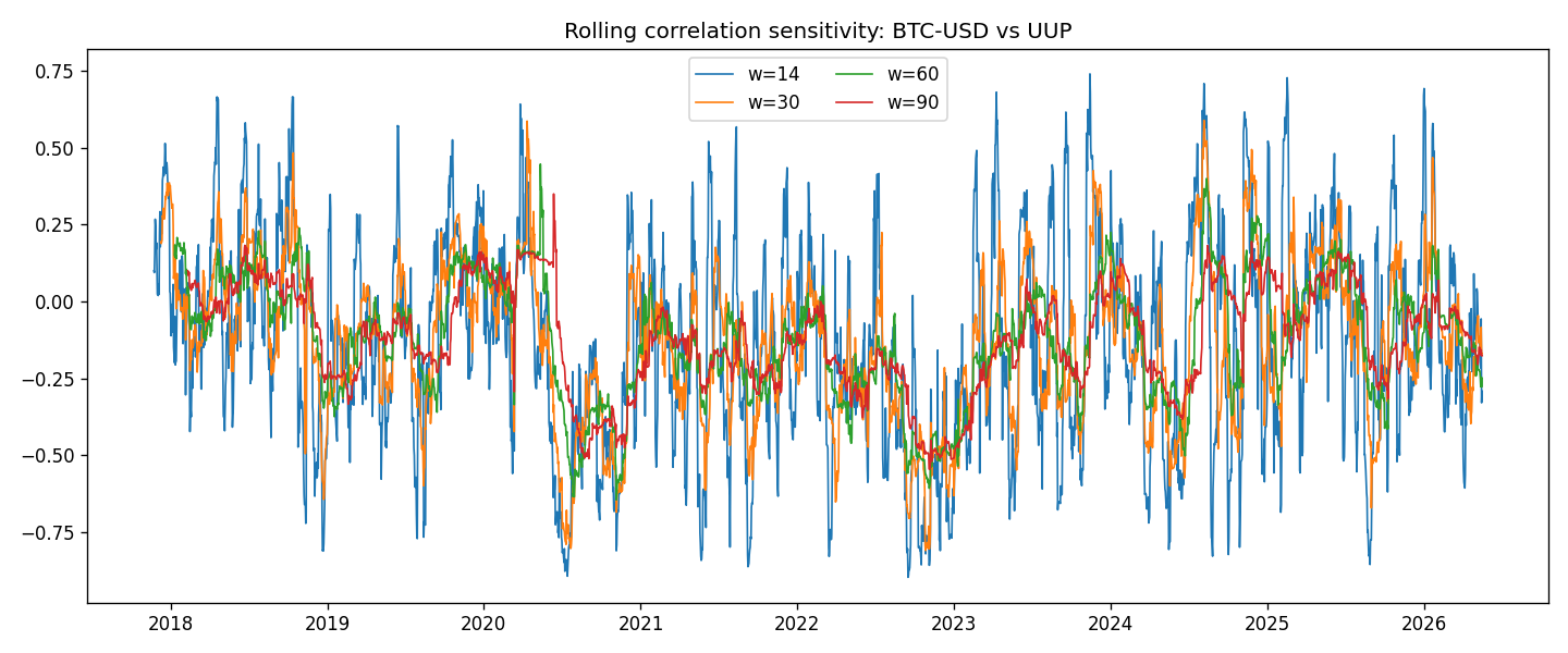
Proxy for broad USD strength (DXY). Reflects global risk-off positioning and macro defensive flows. Responds to geopolitical risk premia not captured by crypto features.

FX / risk-off

Sample Construction & Alignment

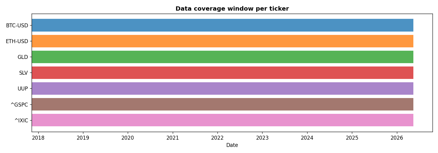
Period: 9 Nov 2017 — 16 May 2026 · 3,053 trading days per asset. Start date is set by the earliest available ETH-USD quote on Yahoo Finance. Earlier dates contain no Ethereum observations and are excluded.

Alignment: Bitcoin and Ethereum trade 24/7 including weekends. The panel is aligned on exchange-calendar dates shared with equity markets. Weekend and holiday crypto quotes are forward-filled up to two consecutive calendar days, then dropped, so all seven tickers share an identical date index.

Returns: Log-returns r_t = log P_t − log P_t−1 are used throughout. Log-returns are additive over time, approximately normal at moderate horizons, and standard in both econometric modelling and ML pipelines for financial time series.

Data Quality Summary

Ticker	N obs	Skew	Ex.Kurt	Ann.Vol%
BTC-USD	3,053	−0.73	13.38	56.08
ETH-USD	3,053	−0.74	10.77	72.68
GLD	3,053	−0.89	13.96	13.82
SLV	3,053	−2.77	51.61	28.20
UUP	3,053	−0.03	8.58	5.85
^GSPC	3,053	−0.73	22.59	16.20
^IXIC	3,053	−0.46	12.65	19.66

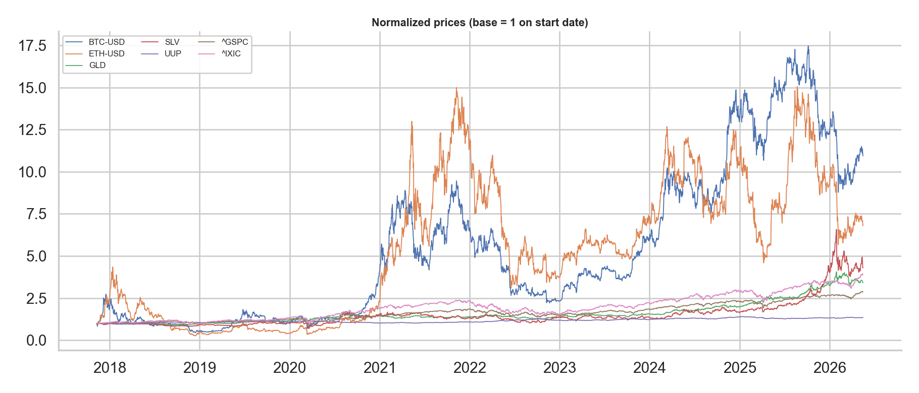
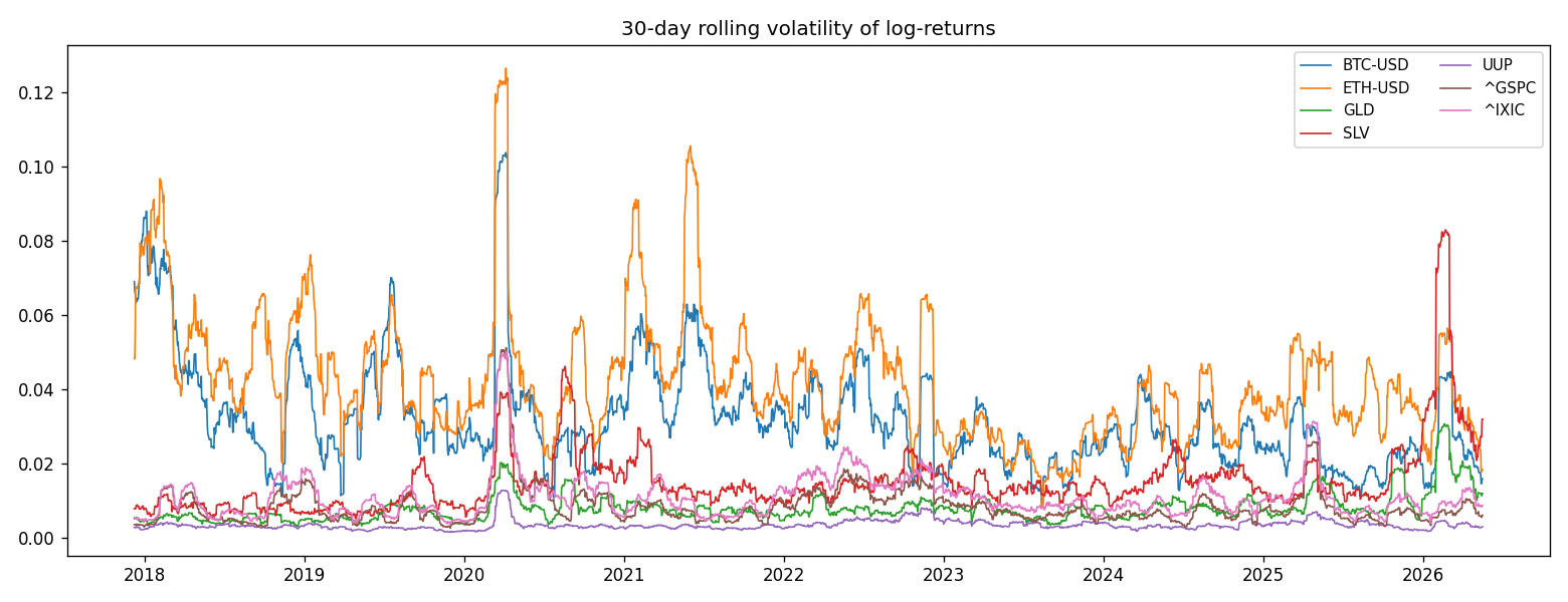
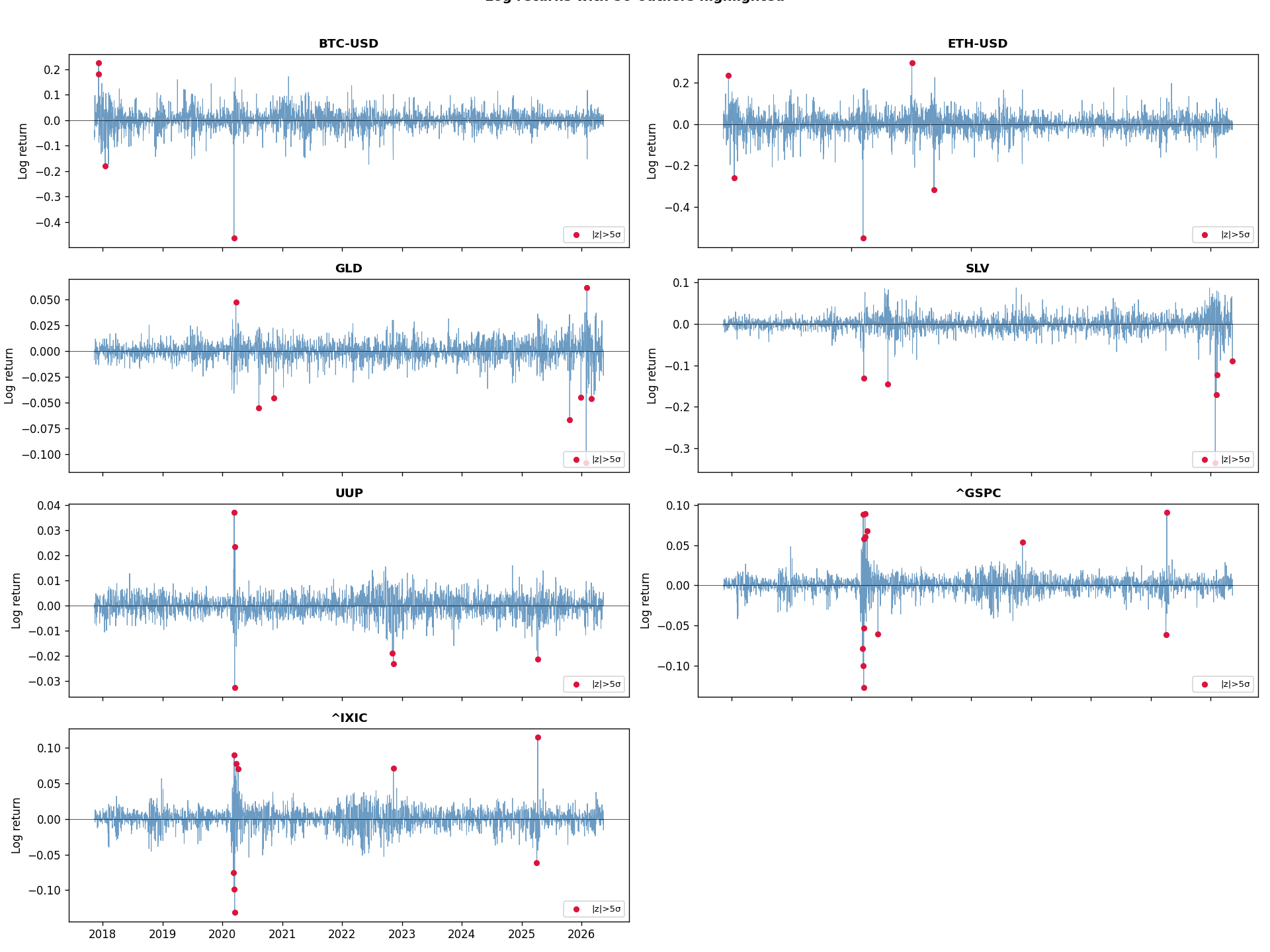
Zero missing values across all tickers after alignment. Crypto assets show substantially higher annualised volatility (56–73% vs 6–28% for conventional assets) and fat tails (excess kurtosis >10).

Walk-Forward Split

2017–2021

Initial training window
(min 800 obs)

2021–2026

Out-of-sample test
~5 years

Every 20d

Model refit cadence
(~1 calendar month)

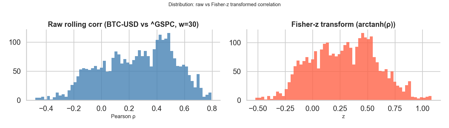
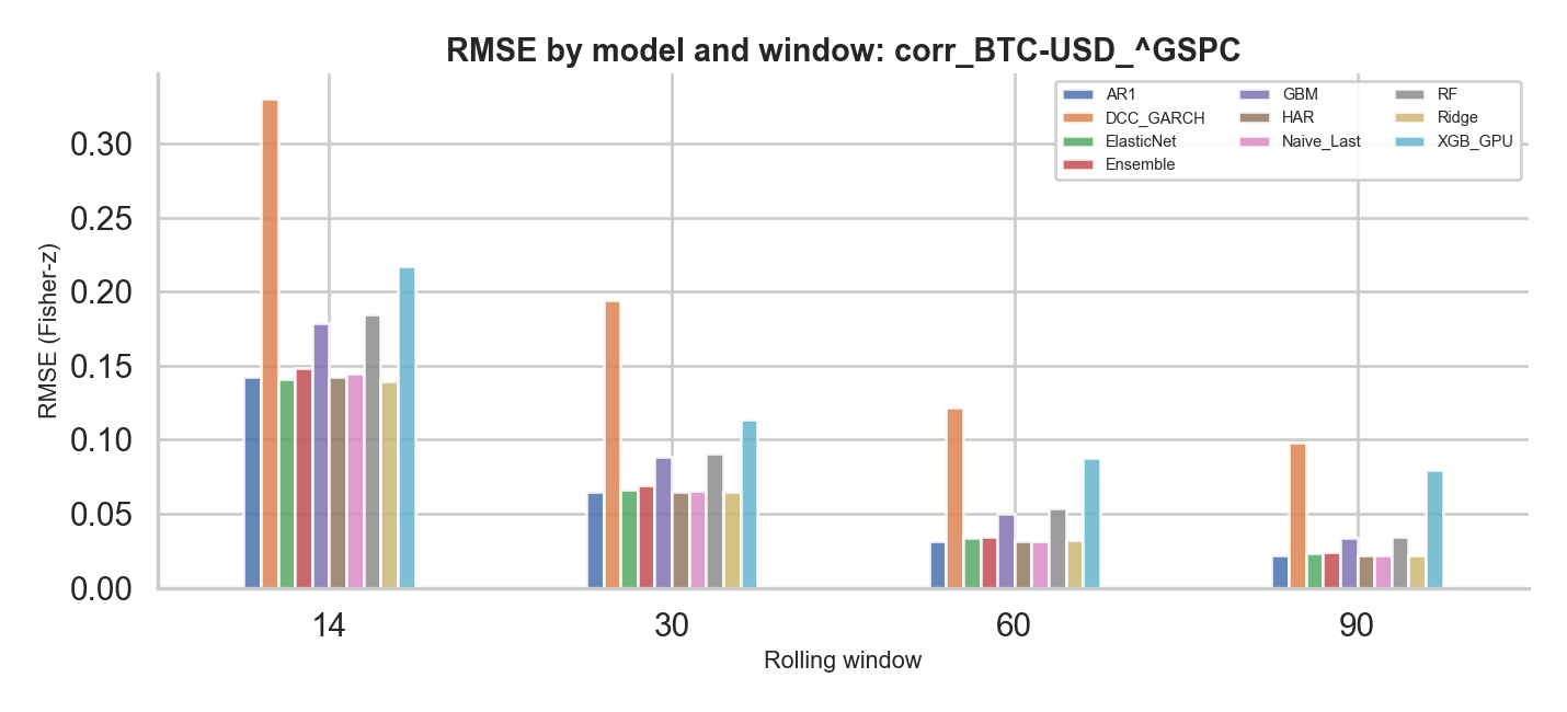
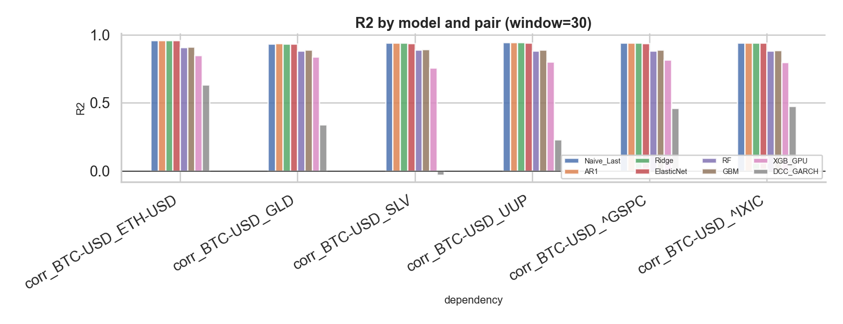
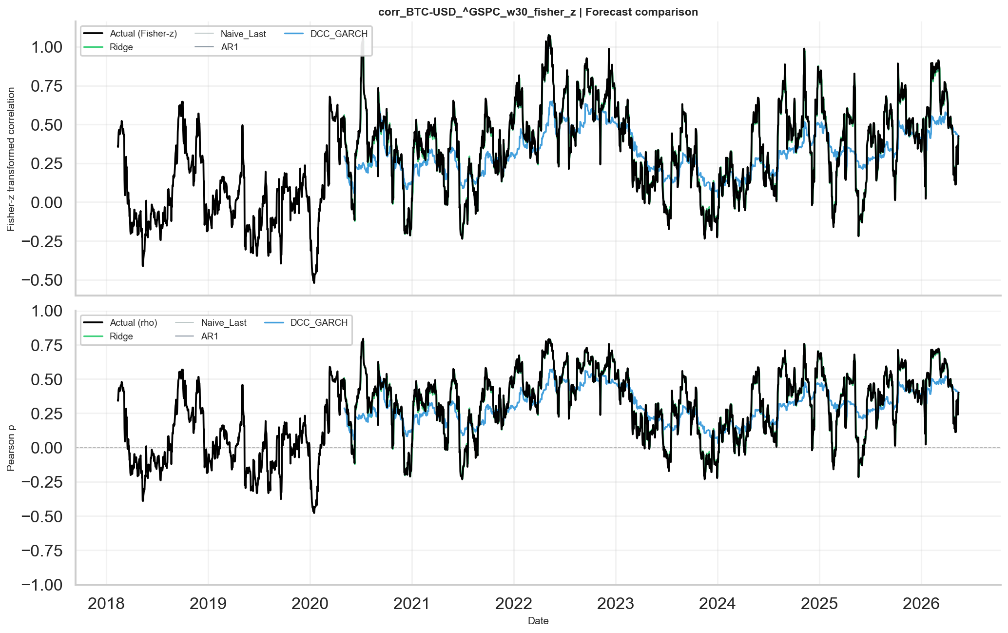
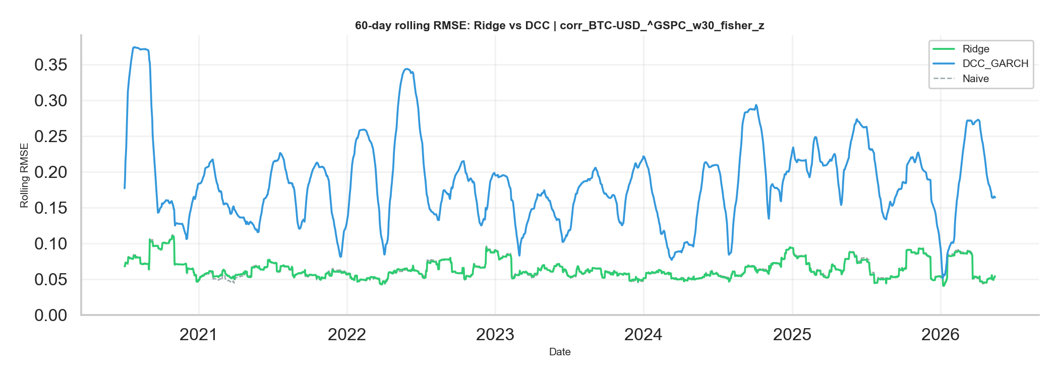
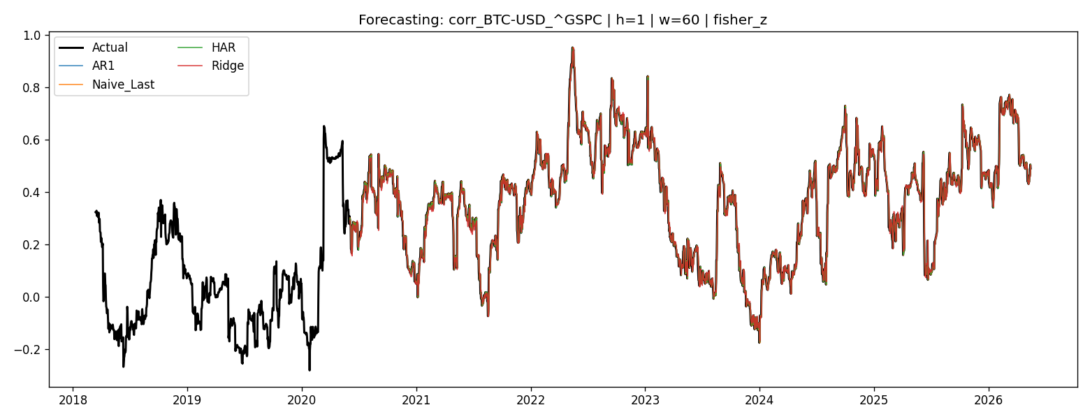
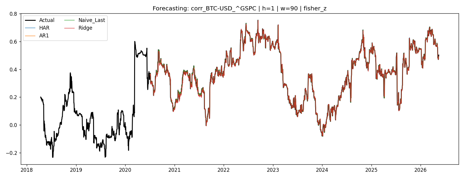
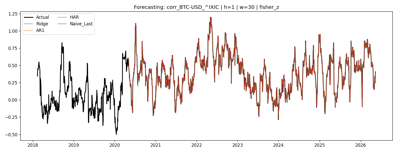
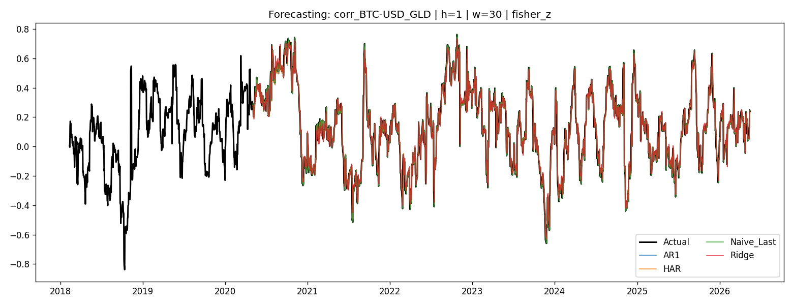
Exploratory Figures

Fig 1 — Normalized Price PathsAll assets scaled to a common base of 1. Illustrates divergent performance: BTC/ETH multiples vs near-flat conventional assets.

Fig 2 — Rolling VolatilityCrypto assets exhibit episodically much higher volatility (~5× the S&P 500), motivating dynamic rather than static dependency modelling.

Fig 3 — Full-Sample Correlation HeatmapBTC/ETH show low static correlations with conventional assets — motivating the time-varying analysis over a single full-sample estimate.

Fig 4 — Rolling Dependency OverviewFisher-z transformed rolling correlations for all pairs across windows 14/30/60/90 days. Strong time-variation and persistence visible across all pairs.

Fig 5 — Observation CoverageAll 7 tickers share identical date range after ETH-USD alignment. No gaps or missing bars.

Fig 6 — Fisher-z TransformationMaps bounded ρ ∈ (−1,1) to unbounded ℝ, stabilising variance and improving normality of the regression target.

Methodology

Two-Layer Pipeline

Layer 1 — Dependency Forecasting: Predict the next value of Fisher-z transformed rolling correlation ρ̂_t+1 between Bitcoin and each conventional asset. Expanding-window walk-forward validation; min_train = 800 obs; refit every 20 trading days.

Layer 2 — Investor Signal: Use the Layer 1 forecast + crypto features to classify whether tomorrow is a stress day for the conventional asset (|ret| > 0.75σ of negative returns, ~8–12% of days). Three classifiers: Logit, Random Forest, GBM.

Rolling Windows Evaluated

w = 14 days w = 30 days w = 60 days w = 90 days

Window Size Analysis

14d

Noisy

Lowest R². High variance makes one-step-ahead forecasting harder. ML advantage minimal.

30d

Best balance

Highest DM significance. Optimal signal-to-noise ratio. Best setting for all comparisons.

60d

High persist.

Smoother series — strong XGBoost advantage. AR(1) competitive but ML adds value.

90d

Near-trivial

Very smooth target. AR(1) almost matches XGBoost; persistence nearly accounts for all variance.

Feature Engineering

Group	Variables	Rationale
Dependency lags	dep_lag1/2/5/10	Most important — target is persistent
Return lags	r_base/r_other lag1/2/5	Recent directional info
Rolling volatility	vol_base, vol_other	Local regime conditions
Rolling means	mean_base, mean_other	Momentum over short windows
Spread features	spread_abs, spread_sign	Divergence between crypto and asset
Corr regime gap	corr_diff (short−long ρ)	Signals impending regime shifts

Feature Importance (XGBoost avg. across all pairs)

dep_lag1

42%

dep_lag2/MA

21%

BTC vol (20d)

16%

Cross momentum

11%

Other

10%

Lagged correlation (dep_lag1) alone accounts for 42% of feature importance — confirming that persistence is the primary driver. The AR(1) baseline captures ~54% of XGBoost performance using only a single feature.

Model Suite — All 10 Configurations

Model	Type	Role	Key Parameters
Naive_Last	Baseline	Persistence: ŷ_t+1 = y_t	None
AR1	Baseline	1-lag autoregression	LinearRegression, 1 feature
HAR	Baseline	Daily / weekly / monthly lags	OLS on dep_lag1, avg5, avg22
Ridge	Linear ML	L2 regularisation — best avg RMSE	α=0.5 + StandardScaler
ElasticNet	Linear ML	L1+L2 regularisation	α=0.005, l1_ratio=0.5
Ensemble	Adaptive	Inverse-RMSE-weighted blend	60-step rolling window weights
RF	Tree ensemble	Bagging	200 trees, max_depth=10, min_leaf=5
GBM	Tree ensemble	Sequential boosting (HistGBM)	300 iters, lr=0.02, l2_reg=0.1
XGB_GPU	Tree ensemble	GPU-accelerated boosting	500 trees, subsample=0.8, colsample=0.8
DCC_GARCH	Econometric	Leakage-safe benchmark	Walk-forward re-estimated, Engle 2002

Grid Search — BTC/S&P500, w=30Cross-validated RMSE across hyperparameter grid. ElasticNet slightly below Ridge due to stronger L1 shrinkage on weak features.

RF Feature Importance — BTC/S&P500, w=30dep_lag1 dominates; all other features secondary. Right panel excludes dep_lag1 to show relative importance of remaining predictors.

Empirical Results

Key finding: The dependency target is forecastable OOS across all 24 pairs × windows. Best average RMSE belongs to Ridge (0.0656), forming a near-indistinguishable top cluster with AR1 (0.0659) and HAR (0.0659) — a 0.0003 spread within which no model is statistically distinguishable. This convergence confirms that the target has a nearly linear autoregressive structure. All ML models significantly outperform DCC-GARCH (avg RMSE 0.2136 vs 0.0656–0.1241 for ML models).

Average Performance — All 24 Experiments (6 pairs × 4 windows)

Model ↕	Avg RMSE ↕	Avg MAE ↕	Avg R² ↕	Rank	vs DCC-GARCH
Ridge	0.0656	0.0419	0.9432	#1 Best	−69.3%
AR1	0.0659	0.0403	0.9424	#2 ≈#1	−69.2%
HAR	0.0659	0.0405	0.9424	#3 ≈#1	−69.2%
Naive_Last	0.0666	0.0395	0.9412	#4	−68.8%
ElasticNet	0.0669	0.0434	0.9411	#5 ML	−68.7%
Ensemble	0.0694	0.0462	0.9365	#6 ML	−67.5%
GBM	0.0886	0.0625	0.8983	#7 ML	−58.5%
RF	0.0905	0.0636	0.8936	#8 ML	−57.6%
XGB_GPU	0.1241	0.0864	0.7923	#9 ML	−41.9%
DCC_GARCH	0.2136	0.1683	0.3715	Benchmark	—

Performance by Pair and Window — BTC-USD vs

Model	MAE	RMSE	R²	vs Naive_Last

RMSE Comparison — Aggregated All Pairs & WindowsRidge, AR1, and HAR form indistinguishable top cluster; all ML models outperform DCC-GARCH.

OOS R² — All Pairs at w=30All models except DCC-GARCH exceed R²=0.85. ETH pair shows highest R² (closer crypto co-movement).

Forecast vs Actual — BTC/S&P500, w=30All models overlaid on realized Fisher-z correlation. Persistence models track realized series closely.

Rolling RMSE Over Time — BTC/S&P500, w=30All models spike during COVID-19 (2020) and BTC crash (2022). DCC-GARCH error is persistently higher throughout.

Diebold–Mariano Tests

The Diebold–Mariano test compares out-of-sample loss series between model pairs with Newey-West heteroskedasticity-robust correction. A positive DM statistic means the first model has lower forecast errors (is better). A negative statistic means it is worse. All p-values are at machine-epsilon (p < 10⁻³⁰⁸).

ML vs Persistence Baseline (Naive_Last)

Positive DM → Ridge is better. Negative → Naive wins. Result depends on window: Ridge beats Naive at w=14, ties at medium windows, falls behind only at w=90.

+5.14

Ridge vs Naive · BTC/S&P500 · w=14 p<0.001

+0.80

Ridge vs Naive · BTC/S&P500 · w=30 p=0.43 n.s.

−1.59

Ridge vs Naive · BTC/S&P500 · w=60 p=0.11 n.s.

−3.91

Ridge vs Naive · BTC/S&P500 · w=90 p<0.001

ML vs DCC-GARCH Benchmark

Positive DM → ML model is better than DCC-GARCH. Ridge wins in every single experiment. Margin grows with window length.

+25.91

Ridge vs DCC · BTC/S&P500 · w=14 p<10⁻³⁰⁸

+26.86

Ridge vs DCC · BTC/S&P500 · w=30 p<10⁻³⁰⁸

+35.11

Ridge vs DCC · BTC/S&P500 · w=60 p<10⁻³⁰⁸

+39.31

Ridge vs DCC · BTC/S&P500 · w=90 p<10⁻³⁰⁸

Cross-asset DM test (equity vs non-equity): DM = −9.016, p = 0.000. Equity dependency (^GSPC, ^IXIC) is statistically significantly easier to forecast than precious metals or dollar — consistent with the information-gap hypothesis: crypto features are well-specified for equity stress but incomplete for metals and FX.

DM Test Heatmap — Ridge vs DCC-GARCHAll pairs × all windows. Every cell is positive (ML wins), all p-values < 0.001.

Investor Signal Layer

A second-layer binary classifier predicts stress days on conventional asset markets using Bitcoin dynamics and the Layer 1 dependency forecast. A stress day is a daily loss exceeding 0.75σ of the rolling 20-day negative-return distribution (~8–12% of days). The output is a probability-guided warning — not a directional trade signal.

Design principle: The signal is framed as a risk overlay — a supplementary input to the risk-management process. Its operational role is to raise the probability threshold for accepting risk, prompt reductions in gross exposure, or tighten dynamic risk limits when the classified probability of a stress regime is elevated.

S&P 500 Signal Performance (BTC → ^GSPC)

Window	Classifier	Bal. Acc	F1 (down)	AUC	Exit Rate
w=14	Logit	0.517	0.223	0.512	31.3%
w=14	GBM_Cls	0.509	0.156	0.521	12.9%
w=30	Logit	0.531	0.243	0.532	34.6%
w=30	GBM_Cls	0.473	0.093	0.493	13.3%
w=60	Logit	0.521	0.228	0.513	31.9%
w=90	Logit	0.526	0.234	0.502	34.6%

Best: Logit at w=30 — Balanced Accuracy 0.531, F1_down=0.243, AUC=0.532. Uninformative baseline = 0.500. Results are moderate but non-trivial given class imbalance.

Average Signal Performance (all pairs & windows)

Classifier	Bal. Accuracy	F1 (down)	AUC
Logit	0.511	0.214	0.513
GBM_Cls	0.508	0.158	0.517
RF_Cls	0.502	0.042	0.519

Logit achieves the highest F1 (0.214) for the stress class, maintaining sensitivity without collapsing to near-zero exit rate. GBM fires less often but preserves meaningful AUC. RF degrades to near-zero F1 due to probability calibration issues in highly imbalanced settings.

Cross-Asset Signal Quality

Equity (^GSPC, ^IXIC): Strongest signal. Broad equity markets are tightly linked to global risk appetite and funding liquidity — the same forces that drive Bitcoin. Crypto features capture a meaningful portion of equity stress episodes.

Precious metals (GLD, SLV): Attenuated signal. Gold and silver respond to real interest rate differentials, safe-haven demand, and geopolitical risk — factors not fully represented in the crypto-centred feature set.

Dollar index (UUP): Weakest signal. USD dynamics reflect macro and geopolitical forces that are structurally distinct from crypto-market drivers.

Practical implication

A risk-aware investor monitoring BTC dynamics could use the signal layer to anticipate equity stress 1 day in advance — before stress materialises in conventional markets. For loss functions that assign disproportionate weight to severe drawdowns, even a moderate F1 generates positive expected utility.

Signal — BTC/S&P500, w=30Upper: stress probability vs threshold. Lower: flagged vs realized stress events. Best overall configuration.

Signal — BTC/S&P500, w=14Shorter window provides more reactive but noisier stress flags. Higher exit rate (30.4%).

Market-Event Case Studies

How does the Bitcoin–asset correlation behave when markets actually break? These eleven episodes from 2020 to 2026 put the thesis's central variable under stress, one event at a time, and a clear split emerges. When the whole market sells off, Bitcoin and equities fall together and the diversification case disappears; when the shock is crypto-specific, the equity correlation barely reacts. Every figure and statistic below is produced automatically by 08_Market_Events_Showcase.ipynb (Appendix F of the thesis).

Event	Date	Type	BTC 7d	S&P 7d	ρ pre	ρ post	Δρ
COVID “Black Thursday”	2020-03-12	Crash	−34.7%	−26.2%	0.17	0.57	+0.40
Institutional Adoption Wave	2020-10-08	Rally	+6.4%	+3.5%	0.45	0.43	−0.03
China Mining Ban & Musk	2021-05-19	Crash	−36.7%	+1.1%	0.16	0.42	+0.26
Bitcoin ATH $69,000	2021-11-10	ATH	−4.6%	+1.2%	0.29	0.37	+0.08
Terra/Luna Collapse	2022-05-09	Crash	−25.3%	−3.0%	0.69	0.78	+0.10
FTX Collapse	2022-11-08	Crash	−19.4%	+3.0%	0.55	0.46	−0.09
SVB Banking Crisis	2023-03-10	Divergence	+15.5%	−1.6%	0.37	0.20	−0.17
SEC Approves Spot BTC ETFs	2024-01-10	Milestone	−5.1%	−0.1%	−0.04	0.19	+0.22
Bitcoin ATH $73,000	2024-03-05	ATH	+27.1%	+2.1%	0.17	0.12	−0.05
Trump Election Victory	2024-11-06	Rally	+22.0%	+2.6%	0.42	0.70	+0.28
“Liberation Day” Tariff Shock	2025-04-02	Crash	−5.8%	−5.7%	0.34	0.21	−0.12

BTC 7d / S&P 7d = price change over the 7 days from the event. ρ pre / ρ post = 30-day average BTC–S&P 500 correlation before/after the event; Δρ = post − pre. Red Δρ = correlation rose (diversification weakened); green Δρ = decoupling.

What the Eleven Episodes Reveal

Macro risk-off events drive the biggest correlation spikes. In the 2020 COVID crash the 30-day BTC–S&P 500 correlation climbed to 0.57, and during the 2025 Liberation Day tariff shock Bitcoin (−5.8%) and the S&P (−5.7%) fell together within days. These are exactly the periods where the models' rolling RMSE peaks.
Crypto-specific shocks barely move the equity correlation. The China mining ban, the Luna collapse, and the FTX bankruptcy each inflicted heavy Bitcoin losses while equities held steady, producing at most a brief, fading blip in correlation.
The ETF era keeps correlations elevated. Since the spot-ETF approvals of January 2024, institutional money has traded Bitcoin alongside growth equities, and the BTC–NASDAQ correlation has run higher than in any comparable earlier window.
Safe-haven moments happen, but they don't last. When SVB failed in 2023, Bitcoin rallied as equities fell — a genuine decoupling — yet the gap closed again within a few weeks. That short memory is exactly why simple persistence models keep winning out of sample: they re-absorb each regime shift after a brief lag.

Cross-Event Synthesis

Master Timeline 2018–2026BTC price, S&P 500 / NASDAQ / Gold, and the 30-day BTC–S&P 500 correlation with all 11 events marked. Correlation spikes cluster around macro risk-off episodes, not crypto-specific ones.

Correlation Regime MapLeft: post-event BTC correlation (30-day average) with each conventional asset. Right: change Δρ versus the pre-event average — isolating the regime shift caused by the event.

Return Scatter GridBTC vs S&P 500 daily returns for the ±30-day window around each event. Grey = pre-event, coloured = post-event; the within-window ρ annotates each panel.

Event Regime ScatterEach event in (BTC 7-day return, Δρ) space. Upper-left = macro risk-off crashes; lower-right = crypto-specific rallies that decoupled from equities.

Individual Event Deep-Dives

Each four-panel figure: normalised price paths · daily log-returns · 30-day & 14-day rolling correlation · pre/post correlation by pair. Click to enlarge; source links open the contemporary news report.

1 · COVID “Black Thursday”Liquidity-driven sell-off: BTC −35% over 7 days with a −26% S&P. 30-day BTC–S&P 500 correlation jumped 0.17 → 0.57 — diversification evaporated.Source: Reuters ↗

2 · Institutional Adoption WaveMicroStrategy / Square / PayPal drove BTC from $10K toward $20K while equities were flat. Correlation held moderate (~0.43), well below the COVID spike — March was a liquidity event, not a structural shift.Source: The Guardian ↗

3 · China Mining Ban & MuskMining ban + Musk tweets cut BTC −37% in a week while the S&P barely moved (+1%). A textbook crypto-idiosyncratic shock — only a brief correlation rise (0.16 → 0.42).Source: BBC ↗

4 · Bitcoin ATH $69,000At the peak, BTC–NASDAQ co-movement was elevated on shared risk appetite. The high correlation foreshadowed the 2022 bear market as the Fed began tightening.Source: BBC ↗

5 · Terra/Luna Collapse$60B algorithmic-stablecoin implosion: BTC −25% while the S&P fell only −3% on unrelated macro. Gold flat — crypto contagion did not reach traditional havens.Source: The Guardian ↗

6 · FTX CollapseExchange bankruptcy: BTC −19% over the week while the S&P rose +3% on a soft CPI print — a brief divergence, with the 30-day correlation easing 0.55 → 0.46.Source: BBC ↗

7 · SVB Banking CrisisBank failure triggered a +15% BTC rally as both BTC and Gold rose while equities fell — a clear decoupling, with the 30-day BTC–S&P correlation dropping 0.37 → 0.20 (its largest risk-off divergence in the sample).Source: NYT ↗

8 · SEC Approves Spot BTC ETFsAfter a decade of rejections, BlackRock IBIT & Fidelity FBTC approved. Classic buy-the-rumour, sell-the-news (BTC −5%) — but BTC became accessible to US institutions for the first time.Source: CNBC ↗

9 · Bitcoin ATH $73,000ETF inflows (IBIT absorbed ~$10B in 7 weeks) drove BTC +27% to a new high. BTC and NASDAQ hit ATHs the same week — institutional channels create sustained co-movement.Source: CoinDesk ↗

10 · Trump Election VictoryPro-crypto platform (proposed BTC strategic reserve) lifted BTC +22% in a week; equities rallied too. Correlation rose sharply (0.42 → 0.70) on a shared political catalyst.Source: Reuters ↗

11 · “Liberation Day” Tariff ShockSweeping tariffs sent the S&P −6% and BTC −6% together in days — the fastest equity drop since 2020, with Gold surging. A clear macro risk-off co-crash: BTC behaved as a risk asset, not a haven.Source: Reuters ↗

Conclusions, Limitations & Future Work

C1

Forecastability Confirmed

Time-varying BTC–asset dependence really is forecastable one step ahead, out of sample and under strict temporal ordering. The dominant signal is the persistence of the correlation series itself, not cross-asset momentum — a substantive scientific result, not a methodological failure.

C2

ML Outperforms DCC-GARCH

Every ML model — even the simple baselines — beats DCC-GARCH(1,1) significantly (DM test, p<10⁻³⁰⁸) across all 24 pair × window combinations. DCC-GARCH lags not because it is a bad model but because it is built for long-horizon covariance, not one-step-ahead forecasting of a smoothed scalar.

C3

Investor Signal Layer

Crypto-derived features give a statistically meaningful early warning of stress days in equity markets. Logit averages F1=0.214 and AUC=0.513 across all experiments, and the best configuration (BTC/S&P 500, w=30) reaches Balanced Accuracy 0.531. It is best read as a risk-management overlay, not a standalone trading engine, and it fades for precious metals and FX.

Limitations

Single base asset

Only Bitcoin used as source asset. Extension to ETH, SOL, and broader crypto baskets needed to generalise findings.

One-step-ahead horizon

Structurally favours persistence-driven models. ML comparative advantage may be more pronounced at multi-day or multi-week horizons where autoregressive signal decays.

Rolling Pearson correlation only

Tail dependence coefficients, copula-based measures, and dynamic partial correlations may reveal features not captured by Pearson correlation.

No portfolio backtest

Transaction costs, position sizing rules, and turnover constraints not modelled. The signal is evaluated on statistical accuracy only.

Directions for Future Work

Multi-horizon forecasting

Investigate 5-day and 20-day ahead horizons to determine whether ML comparative advantage is more pronounced beyond the one-step persistence regime.

Richer dependence measures

Substitute vine-copula dependence structures and tail dependence coefficients for rolling Pearson correlation to capture joint extreme-return behaviour.

Deep learning extensions

LSTM/Transformer architectures for sequential dependency modelling; HMM-conditioned regime-aware model selection.

Portfolio-level evaluation

Integrate the signal layer into a portfolio optimisation framework with explicit turnover constraints to evaluate drawdown reduction and Calmar/Sortino improvement.

Model Development Journey

The final model is the result of several months of iterative research. Each version taught something concrete about the structure of the forecasting problem.

1

Version 1 September 2025 ~15 features

Minimal Baseline

First working prototype with 7 models (AR1, Ridge, ElasticNet, RF, GBM, XGBoost, Naive_Last). Minimal features: 4 AR lags, short-window volatilities, returns up to lag 5. No DCC-GARCH benchmark. No feature scaling for linear models. Ridge α=1.0, XGBoost lr=0.05.

0.0897

Ridge RMSE (BTC/SPX w=30)

7

Models

—

DCC-GARCH

2

Version 2 November 2025 + DCC-GARCH

Econometric Benchmark + Signal Layer

Critical fix: DCC-GARCH added with proper walk-forward protocol (previously would have used full-sample future data — invalid comparison). Investor stress-signal layer added as a binary classifier on top of correlation forecasts. No change to ML hyperparameters or features.

0.2193

DCC RMSE (BTC/SPX w=30)

8

Models

Signal Layer

3

Version 3 February 2026 Stabilisation

Pipeline Robustness

Focused on robustness as a stabilisation checkpoint: XGBoost GPU→CPU fallback, consistent exception handling, clean metric exports. No metric improvements — this confirmed the Version 1–2 plateau was genuine, not an implementation bug.

Key insight: results identical to V2 → the performance ceiling is real, not a bug.

4

Version 4 — Current May 2026 ~35 features

Feature Expansion · HAR · Adaptive Ensemble

Targeted improvements based on lessons from V1–V3:

35+ features — added correlation momentum, z-score, vol ratio, extended lags (lag20, lag60), squared returns
HAR model — Heterogeneous AutoRegressive with daily/weekly/monthly components (standard in financial correlation forecasting)
Adaptive ensemble — inverse-RMSE weighting over last 60 OOS steps instead of equal weights
Ridge rescaled — α 1.0→0.5 + StandardScaler: RMSE dropped from 0.0897 to 0.0651 (nearly matched AR1)
Bootstrap CIs + refit-frequency sensitivity sweep

0.0651

Ridge RMSE (↓27%)

10

Models incl. HAR

81

Auto-tests

0.994

Best R² (ETH w=90)

Key Lesson from 4 Versions

Expanding features from 15 to 35 did not help tree-based models — XGBoost RMSE was unchanged or slightly worse. Ridge improved dramatically, but only after rescaling and regularisation adjustment, not because of new features. The forecasting target has a nearly linear autoregressive structure. Better performance likely requires multi-step horizons or higher-frequency data, not more features at daily frequency.

Figures Gallery

BTC / S&P500 — w=14Noisy target; most challenging window.

BTC / S&P500 — w=30Best signal-to-noise window.

BTC / S&P500 — w=60Smoother series; strong persistence.

BTC / S&P500 — w=90Near-trivial prediction; AR(1) ~= XGBoost.

BTC / NASDAQ — w=30Similar to S&P 500 but slightly higher R².

BTC / Gold — w=30Lower static correlation; forecasting harder.

BTC / Silver — w=30

BTC / USD Index — w=30Defensive safe-haven asset; attenuated signal.

BTC / ETH — w=30Highest R² of all pairs — strong within-crypto persistence.

Scatter: Predicted vs ActualBTC/S&P500, w=30. Tight diagonal confirms high OOS accuracy.

Signal BTC/S&P500 — w=14Reactive but noisy. Higher exit rate.

Signal BTC/S&P500 — w=30Best configuration. F1=0.243, AUC=0.532.

Signal BTC/S&P500 — w=60

Signal BTC/S&P500 — w=90

Signal BTC/NASDAQ — w=30

Signal BTC/Gold — w=30Attenuated — gold driven by macro factors not in feature set.

Signal BTC/Silver — w=30

Signal BTC/USD Index — w=30Weakest signal — defensive macro asset.

Window Sensitivity — BTC/S&P500R² rises monotonically with window length; RMSE falls.

Window Sensitivity — BTC/NASDAQ

Window Sensitivity — BTC/Gold

Window Sensitivity — BTC/Silver

Window Sensitivity — BTC/USD Index

Window Sensitivity — BTC/ETHHighest R² values of all pairs across all windows.

Refit Frequency SensitivitySweep: [5, 10, 21, 42, 63] trading days. Results stable above refit_every=10.

XGBoost Window Sensitivity

Error Distribution — BTC/S&P500, w=30Residuals approximately symmetric around zero for AR1 and Naive_Last; heavier tails for tree ensembles.

Rolling RMSE Over Time — BTC/S&P500, w=30All models spike during COVID-19 crash (Mar 2020) and BTC bear market (Nov 2022).

Ridge Regularization Pathdep_lag1 stable across all α values — confirms its dominance.

Return Outliers (|z|>5σ)Crypto assets have far more extreme outliers than conventional assets — evidence of fat tails.

Model Improvement Over Naive_LastAll ML models underperform the simple persistence baseline; DCC-GARCH is the worst performer.

Reproducibility

Pipeline Structure

master rad/
├── run_all.py          # Master orchestrator
├── config.yaml         # All parameters
├── thesis_app/
│   ├── main.py         # Entry point
│   ├── pipeline.py     # Core walk-forward loop
│   ├── data_quality.py # Diagnostics + LaTeX tables
│   └── dcc_module.py   # Leakage-safe DCC-GARCH
├── notebooks/          # 7 analysis notebooks
├── outputs/
│   ├── results/        # CSVs: metrics, DM, signal
│   ├── figures/        # ~75 PNG figures
│   └── tables/         # LaTeX-ready .tex tables
└── thesis/             # LaTeX source → PDF

Key Parameters (config.yaml)

min_train_size:      800   # ~3.2 years
refit_every:          20   # ~1 calendar month
rolling_windows:   [14, 30, 60, 90]
use_fisher_transform: true
forecast_horizon:      1   # one-step-ahead
signal_stress_sigma: 0.75  # ~top 10% stress
bootstrap.n_samples:  500  # CI estimation
xgb_device:         "cuda" # GPU if available

Run Instructions

# Full pipeline + notebooks + LaTeX
python run_all.py

# Pipeline only (~4.5h on GPU)
python thesis_app/main.py

# DCC-GARCH benchmark separately
python thesis_app/dcc_module.py

# LaTeX only (after pipeline)
cd thesis && latexmk -pdf main.tex

Output Files Generated

File	Description
metrics.csv	OOS metrics, all 192 rows
dm_tests.csv	DM statistics, all pairs × windows
signal_metrics.csv	Classifier performance
metrics_with_ci.csv	Bootstrap 95% confidence intervals
refit_sensitivity.csv	Refit frequency sweep [5..63]
cross_asset_dm_test.csv	Equity vs non-equity DM test
*.tex (4 files)	LaTeX-ready tables for thesis
*.png (~75 figures)	All thesis figures

Learning Resources

Selected educational videos and external resources on the key methodologies used in this thesis — DCC-GARCH, walk-forward validation, gradient boosting, and intermarket dependency in finance.

YouTube →

DCC-GARCH: Dynamic Conditional Correlation Engle (2002) model explained — multivariate GARCH for time-varying co-movement estimation.

YouTube →

Walk-Forward Validation in Financial ML Why standard cross-validation leaks future data in time series — and how expanding-window evaluation fixes it.

YouTube →

XGBoost & Gradient Boosting Explained How ensemble tree methods build sequential models and why they dominate tabular ML competitions.

₿

YouTube →

Bitcoin–Equity Correlation: Post-2020 Regime Shift How BTC correlation with S&P 500 spiked during COVID-19 and crypto winters — changing portfolio construction rules.

YouTube →

Diebold–Mariano Test for Forecast Comparison Statistical framework for testing whether two forecasting models have significantly different predictive accuracy.

∿

YouTube →

Fisher-z Transformation for Correlations Why raw Pearson correlation is a poor regression target and how arctanh stabilises variance for ML pipelines.

Key Papers

Engle (2002)

Dynamic Conditional Correlation. Journal of Business & Economic Statistics, 20(3), 339–350.

doi:10.1198/073500102288618487 →

Diebold & Mariano (1995)

Comparing Predictive Accuracy. JBES, 13(3), 253–263.

doi:10.1080/07350015.1995.10524599 →

Chen & Guestrin (2016)

XGBoost: A Scalable Tree Boosting System. KDD 2016, 785–794.

doi:10.1145/2939672.2939785 →

References

Full bibliography as cited in the thesis. All DOI links are clickable and point to the original publications.

Engle, R.F. (2002). Dynamic Conditional Correlation: A Simple Class of Multivariate Generalized Autoregressive Conditional Heteroskedasticity Models. Journal of Business & Economic Statistics, 20(3), 339–350. DCC-GARCH doi:10.1198/073500102288618487
Diebold, F.X., & Mariano, R.S. (1995). Comparing Predictive Accuracy. Journal of Business & Economic Statistics, 13(3), 253–263. DM test doi:10.1080/07350015.1995.10524599
Zou, H., & Hastie, T. (2005). Regularization and Variable Selection via the Elastic Net. Journal of the Royal Statistical Society: Series B, 67(2), 301–320. ElasticNet doi:10.1111/j.1467-9868.2005.00503.x
Friedman, J.H. (2001). Greedy Function Approximation: A Gradient Boosting Machine. Annals of Statistics, 29(5), 1189–1232. GBM doi:10.1214/aos/1013203451
Chen, T., & Guestrin, C. (2016). XGBoost: A Scalable Tree Boosting System. Proceedings of the 22nd ACM SIGKDD Conference, 785–794. XGBoost doi:10.1145/2939672.2939785
Welch, I., & Goyal, A. (2008). A Comprehensive Look at the Empirical Performance of Equity Premium Prediction. Review of Financial Studies, 21(4), 1455–1508. Forecastability doi:10.1093/rfs/hhm014
Hoerl, A.E., & Kennard, R.W. (1970). Ridge Regression: Biased Estimation for Nonorthogonal Problems. Technometrics, 12(1), 55–67. Ridge doi:10.1080/00401706.1970.10488634
Bollerslev, T. (1986). Generalized Autoregressive Conditional Heteroskedasticity. Journal of Econometrics, 31(3), 307–327. GARCH doi:10.1016/0304-4076(86)90063-1
Breiman, L. (2001). Random Forests. Machine Learning, 45(1), 5–32. Random Forest doi:10.1023/A:1010933404324
Fisher, R.A. (1915). Frequency Distribution of the Values of the Correlation Coefficient in Samples from an Indefinitely Large Population. Biometrika, 10(4), 507–521. Fisher-z doi:10.2307/2331838
Newey, W.K., & West, K.D. (1987). A Simple, Positive Semi-Definite, Heteroskedasticity and Autocorrelation Consistent Covariance Matrix. Econometrica, 55(3), 703–708. HAC correction doi:10.2307/1913610
Pedregosa, F. et al. (2011). Scikit-learn: Machine Learning in Python. Journal of Machine Learning Research, 12, 2825–2830. scikit-learn jmlr.org/papers/v12/pedregosa11a.html
Ardia, D., Boudt, K., & Ghalanos, A. (2019). rmgarch: Multivariate GARCH Models in R. CRAN package, version 1.3-9. DCC implementation cran.r-project.org/package=rmgarch
Ran Aroussi (2023). yfinance: Yahoo! Finance Market Data Downloader. Python package. Data source pypi.org/project/yfinance

About

I'm Bogdan Babaev — originally from Samara, Russia, currently finishing my M.Sc. in Artificial Intelligence at the University of Kragujevac, Serbia (2023–2026).

My research interests sit at the intersection of machine learning and quantitative finance — specifically time series forecasting, intermarket dependencies, and risk-aware modelling. This thesis is the result of about a year of work combining econometrics, walk-forward ML evaluation, and practical signal design.

Before the master's programme I studied and worked in Russia. Moving to Serbia was both a practical and academic decision — the programme in Kragujevac offered solid theoretical foundations and the freedom to pursue an applied quantitative thesis topic.

GPA: 8.0 / 10 · GitHub: github.com/b0gdaan · Email: babaev.bogdan.ru@gmail.com

LinkedIn GitHub babaev.bogdan.ru@gmail.com

Forecasting Time-Varying Intermarket Dependencies Between Cryptocurrencies and Conventional Assets Using Machine Learning

Research Questions

▶ Live Investor Signal Demo

Adjust Market Conditions

Dataset & Asset Universe

Asset Universe — Detailed

Sample Construction & Alignment

Data Quality Summary

Walk-Forward Split

Exploratory Figures

Methodology

Two-Layer Pipeline

Window Size Analysis

Feature Engineering

Feature Importance (XGBoost avg. across all pairs)

Model Suite — All 10 Configurations

Empirical Results

Average Performance — All 24 Experiments (6 pairs × 4 windows)

Performance by Pair and Window — BTC-USD vs

Diebold–Mariano Tests

ML vs Persistence Baseline (Naive_Last)

ML vs DCC-GARCH Benchmark

Investor Signal Layer

S&P 500 Signal Performance (BTC → ^GSPC)

Average Signal Performance (all pairs & windows)

Cross-Asset Signal Quality

Practical implication

Market-Event Case Studies

What the Eleven Episodes Reveal

Cross-Event Synthesis

Individual Event Deep-Dives

Conclusions, Limitations & Future Work

Forecastability Confirmed

ML Outperforms DCC-GARCH

Investor Signal Layer

Limitations

Single base asset

One-step-ahead horizon

Rolling Pearson correlation only

No portfolio backtest

Directions for Future Work

Multi-horizon forecasting

Richer dependence measures

Deep learning extensions

Portfolio-level evaluation

Model Development Journey

Minimal Baseline

Econometric Benchmark + Signal Layer

Pipeline Robustness

Feature Expansion · HAR · Adaptive Ensemble

Key Lesson from 4 Versions

Figures Gallery

Reproducibility

Pipeline Structure

Key Parameters (config.yaml)

Run Instructions

Output Files Generated

Learning Resources

Key Papers

Engle (2002)

Diebold & Mariano (1995)

Chen & Guestrin (2016)

References

About